
Please, read the file, readme.txt, that came with SAR Image Processor.
Because this is a single page manual that contains many images, it may take a long time to download. The advantage to having everything on one page is that you can use your browser's Find function to serve as an index. To save time with future viewing of this manual, you should save this web page as an MHT file on their hard disk. Then, you can refer to this MHT file and need only occasionally check this web page for changes.
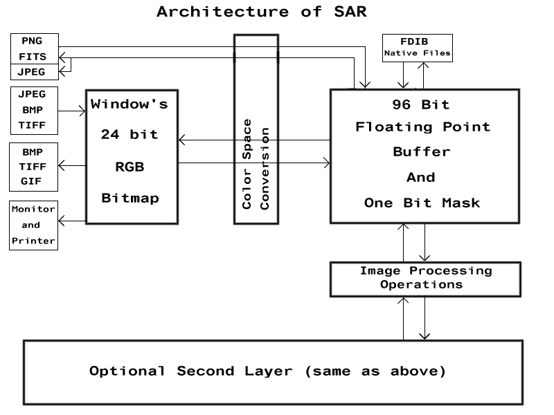
SAR is unusual because it uses a 32 bit/channel floating point buffer. See Figure 1. The main advantage of this is that operations with inverses can be incrementally applied to an image without accruing significant round off and clipping errors. Also, the floating point buffer allows images to be saved in 48 (and greater) bit image files without loss of accuracy. The primary disadvantage is that large amounts of RAM are needed; however, the price of RAM is low and dropping. The user has options to destroy the floating point buffer, or not create a floating point buffer upon opening an image file. All resize operations, except IFS, remain operative, thereby substantially reducing RAM requirements for enlargements.
Another unusual aspect of SAR is that it has a relatively small number of operations and a large number of color space modes. SAR can do many things that other image editors can by using some combination of operation and color space. One advantage of this reduced instruction set is that a user should have no trouble locating a menu item. There are no submenus, i.e., all menus are one deep.
Clicking on certain menu items will automatically program the F2/F3 keys for an operation/inverse. Then, the F2 and F3 keys can be pressed as often as desired to obtain a desired effect. Pressing F3 cancels the effect of F2 and vice versa. Also, whenever possible, Shift+F2 and Shift+F3 will apply 10 times the effect, whereas Ctrl+F2 and Ctrl+F3 will apply 1/10 the effect. Operations without inverses normally take effect as soon as their menu items are clicked; however, almost any operation can be programmed into F2 by holding down the Ctrl key while clicking on the menu item. (The Ctrl key should be pressed down while the client window has focus and released after the menu item is clicked.) The name of an F2/F3 operation appears on the menu bar after Help. Previously programmed F2/F3 operations can be scrolled with keys < and >. Only operations loaded into the F2 key can be directly applied as a Batch operation on files. However, sequences of up to 32 F2, F3, Shift+F2, Shift+F3, Ctrl+F2 and Ctrl+F3 pressings, along with parameter settings, can be recorded as a "Program." This "Program" can be loaded into F2 and then applied to batch files. Also, the "Program" can be saved as a *.sar file.
Regarding the Properties Dialog Box (Q key), Figure 2, all properties set with this dialog are saved in the file, sar.ini, when the program closes and read when the program opens. The tree structure on the left corresponds very roughly to items as they appear on the menu bars. The dialog box is navigated by clicking on a tree item. As a default, the option, Automatic Query of Properties, is set. With this option, whenever a menu item is clicked, the dialog box will automatically appear with the relevant item on the tree already active. From this, you can learn the locations on the tree structure that affect a menu item. After you become familiar with these locations on the tree, you can turn off Automatic Query of Properties by pressing Ctrl+Q, and just set the properties (via Q key) when needed. At any time, the properties can be reset to default values with Options>"Set Properties to Default."
Set defaults under Options and open a small image file. Use arrow keys to position image on screen (For fine control, us numeric keypad's 2, 4, 6, 8 keys) Left click the cursor on any pixel in the image and view the pixel information, (x,y)(R,G,B)(X,Y,Z), in the status bar. The coordinates (x,y) have an origin at the lower left corner of the image. The 8 bit RGB values (R,G,B) are stored in the bitmap. These RGB values are integers that can only vary between 0 and 255. This is what your Printer and Monitor sees. (X,Y,Z) are the color space intensities for the color channels stored in the floating point buffer. Press F8 to show the histogram. The red graph represents the X channel, the green represents the Y channel, and the blue represents the Y channel.
Observe the last item on the menu bar with default text "NoOp"("NoOp" stands for "No Operation."). This represents the operation applied with the F2/F3 keys. Click menu item, Basic>"Set F2, F3 to Add/Subtract a Constant". You will automatically be queried for optional entry of a parameter. Leave the default and click OK or press Enter key. "Add/Sub Const" will appear on the menu bar replacing "NoOp." Press F2 and watch the histogram shift right and the image brighten. Press F3 and watch the the histogram shift left and the image darken. This operation is equivalent to a conventional brightness control. Now, open menu CSpace and uncheck Channel Y and Channel Z, leaving only Channel X checked. (The menu won't disappear until you press F10 key or click elsewhere. Also, channel selection can be made using keys 1, 2, and 3 and the selection status can be read on the third pane of the status bar.) Pressing F2/F3 will now only affect the X channel. To disable this without reselecting channels, press the F4 key and "Cond( On)" will change to "Cond(Off)" on the menu bar. This controls whether an operation is applied conditionally with respect to channel selection and masking.
Change back to "Cond( On)" and make sure that all channels are active. Press F1 (refresh), and repeat above with Basic>"Set F2, F3 to Multiply/Divide a Constant." The histogram expands/contracts to the right. This is similar to, but not exactly equivalent to, conventional contrast control.
To get conventional contrast control, requires two steps. First, click Queue>"Enter Median Color." The median color of the entire image will be entered into the top of the Queue (which can be observed on the menu). Second, click Basic>"Set F2/F3 to Interpolate/Extrapolate Color." Now, pressing F2/F3 will contract/expand the histogram distributions about their medians. This is conventional contrast control.
Change color space modes by checking CSpace>HSV and set the channels so that only "Channel Y = S" is checked. Observe that the histogram changes but the image stays the same. Return to "Mul/Div Const" (Press key < for previously entered settings and key > for later entered settings). Now pressing F2/F3 will increase/decrease the color saturation of the image.
Repeat with "Add/Sub Const" and the H channel. By now, you should get the idea behind SAR.

Creates an additional window. It should be noted that, unlike some other software, SAR does not automatically open an image in a new window. In combination with synchronized scrolling, multiple windows are most useful for side by side comparison of similar images.
With this option checked, no floating point buffer will be created when an image file is read. The purpose of this is to conserve RAM for interpolation operations. With this option checked, SAR will not read or write file formats greater than 24 bit. Most operations, other than some resizing operations and printing, will be disabled without a floating point buffer. Also, it is sometimes possible to create images that are too large to save. (As Microsoft code contained in the GDIPLUS.DLL is used for 24 bit files, I blame Microsoft.)
SAR now reads 24 and 48 bit integer and 96 bit floating point TIFF subformat. SAR normally reads 24 and 48 bit PNG. SAR reads a proprietary IFS format for image enlargement that will be discussed under Resize.
Select multiple files in dialog box by holding down the Ctrl key. The F2 programmed operation will be applied to each file and (*except for two circumstances) saved. Overwriting can be avoided by attaching a suffix to every file name. During processing, the number of images is counted in the fifth pane of the status bar. The user can control the file buffer size by setting the parameter, Maximum Characters. A larger buffer size will be necessary to read a sufficiently large file list. If you encounter a failure, it may be easier to test the adequacy of a larger setting by using rather than Batch Operation, since this feature is shared.
*A processed image is not saved when F2 is programmed with Print or recorded actions ending with Print.
Initially, multiple selections are made from a dialog box by holding down the Ctrl key, after which, each time key F9 is pressed, a new file is loaded from that selection until the sequence is completed. You can back up by pressing Shift+F9. The sequence can be prematurely terminated by pressing Ctrl+F9, or holding down the Ctrl key before clicking menu item. The number of images is counted in the fifth pane of the status bar. If the sequence terminates prematurely, it is probably because the size of a buffer which holds file names was exceeded. To fix this problem, increase the buffer size by setting the shared Batch parameter, Maximum Characters.
Use this after Sequential Load above to automatically display the images at a specified time interval in between. For example, with Irfanview, you can decompile an MPEG file into still frame BMP files. Using SAR's batch capability, you can retouch and enlarge these frames. Then you can use Animate Sequence for a better animated visual display than with the original MPEG.
There is no "Save" because it is generally bad practice to overwrite image files. This is particularly true with SAR because EXIF information is lost. Unlike with other programs, using "Save As," will not make the saved file the active file. Also, when closing SAR, there is no dialog box asking whether you want to save the image.
SAR's native format is the FDIB (*.fdib) file, which contain information about the color space, channel selection, and mask. FDIB is the only file type that can change the color space and channel settings when the file is opened.
There are five image file formats that have property settings:
This is the closest thing to a conventional "Undo". (SAR has no conventional, Ctrl+Z, undo, because writing images to disk in 32 bit floating point format takes too much time to make it automatic.) These are for convenient storage and recall of intermediate results during image processing. Shift+F11 and Shift+F12 respectively stores images to files, SAR.FDIB and SAR2.FDIB, in the same directory that SAR is installed. Beware, these files can be very large and they are not automatically deleted when SAR closes. Pressing F11 and F12 loads these files.
These functions are self explanatory, except to say that they have been included to save steps in writing actions.

Important Note: The settings for the Page Setup Dialog (e.g., margin settings, paper size) and the Printer Properties Dialog (e.g., paper type) are not preserved when SAR closes. Whenever SAR opens, these settings will be the defaults which the user can set via the Windows OS. However, such settings, once made in SAR, will persist until SAR closes. Also, there is a "bug" under Windows ME (and probably 98 and 95), but not XP, in which a sufficiently large image may fail to show in the preview window of the Page Setup dialog box. This bug does not affect printing.
Automatic interpolation to optimum size for printing via Lanczos or Triangulation will usually result in better prints than using the interpolation built into the printer driver. However, for superior results, I recommend that images first be enlarged 4X by edge preserving methods such as Jensen-Xin Li hybrid or IFS. This can be done by composing an action. That action can be used by pressing the F2 key or it can be used for batch processing.
The steps for making the action are as follows:
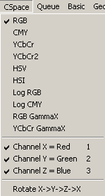
The status of a color space selection is indicated in the second pane of the status bar and as check marks in the menu.
This is the default mode. SAR's RGB is similar to conventional RGB except intensity values less than zero and greater than 255, as well as non integral values, are allowed. As with all SAR color spaces, appropriate clipping and rounding to integer values is performed outside of the floating point buffer.
There are slightly different standards for YCbCr because the calculation is based on the characteristics of various phosphors use color television and monitors. SAR uses basically the same standard that JPEG, TIFF, and PNG uses. Interestingly, this is based on phosphors used in late 1950s' television.
Roughly speaking, brightness is represented by Y (Luminance) and color is represented by Cr and Cb. More specifically, Y = 0.2990*R + 0.5870*G + 0.1140*B where R, G, B are RGB channel values. Setting the Cr and Cb intensities of all pixels to zero will result in a grey scale (BW) image. Multiplying the Cr and Cb intensities by a number greater than one, e.g., 1.1, will increase the color saturation. The terms "roughly speaking" are used here because results will differ from those produced by other methods. This color space can be used with some interpolation methods to an advantage. Also, the Cr and Cb channels are often useful in conjunction with Mask>"Set F2, F3 to Mask by Color."
Similar to YCbCr, except Y = (R+G+B)/3.
H is the hue which varies cyclically from 0 to 360 degrees. Red is 0, green is 120 and blue is 240. S is color saturation and normally varies between 0 and 1. V, another measure of brightness, stands for "value" and simply represents the maximum R, G, an B value and therefore normally varies between 0 and 255. Again, the range for these numbers has been increased in the floating point buffer. The hue of a color of saturation zero (black, grey and white) has been arbitrarily defined as 0 (red). For that reason, do not use any operation on the S channel that will make previously zero values positive. Otherwise, white areas will become pink or red. Multiplication and Gamma are safe to us on the S channel. Do not use HSV with interpolation!
Similar to HSV, except I, intensity, represents the average of RGB values. Also, there are subtle differences between the H and S components of HSI and HSV. Do not use this with interpolation!
Adding two images in this color space produces a result identical to that of overlaying two transparencies of the images. White is completely transparent and black is completely opaque. If you want to add text to an image, just add a black and white text image.
Performs a gamma transformation with a gamma value that can be selected under Miscellaneous.
Performs RGB Gamma transformation before converting to YCbCr.
With "Cond( On)" on the menu bar, certain operations will only be applied to checked channels. When one of these menu items is clicked, the pop up menu will automatically reappear. Pressing the F10 key or clicking elsewhere, e.g., another menu item, will close the menu. Color space selections can also be made using keys, 1, 2, and 3. The selection status can also be read in the third pane of the status bar.

Displays and/or stores coordinate and/or color information for use with the following operations:
When only one point or color is involved, the checked queue color applies. When multiple or variable points or colors are involved, they are applied from the top of the queue. Coordinate and/or color information can be entered in three ways:
First, by left clicking on an image pixel and pressing the Enter key. This will place the pixel information on the top of the queue. Previously entered values are shifted downward.
Second, coordinate and color information can be manually edited from dialogs. Holding down the Shift while clicking on the menu item will bring up the coordinate dialog. Similarly, the Ctrl key will bring up the color dialog. Enter numbers separated by commas.
Third, the following three operations enter colors into the queue.
The average color for an image area is placed into the queue. Normally, this area applies to the entire image, but this can also be an unmasked area or a painted area. When this operation is applied by clicking on the menu, the menu will reappear so that you can examine the color at the top of the queue. You can close the menu by pressing F10 or just clicking elsewhere.
Similar to Enter Average Color. Average is replaced by median.
Similar to Enter Average Color. Average is replaced by wmmr.
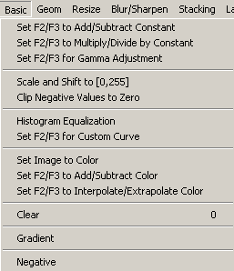
Self explanatory. In RGB space, this can be used to adjust brightness.
Self explanatory. In RGB space, this is similar to contrast control.
Reshapes the histogram by exponentiation of intensity values. Roughly speaking, in RGB space, F2 darkens while increasing contrast and color saturation, F3 lightens the image while decreasing contrast and color saturation. In other color spaces, you need to study the effect.
Produces maximally flat histogram (subject to some constraints).
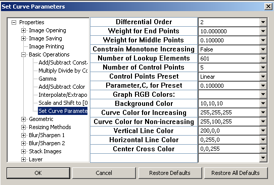
The following dialog box will appear:
afterwhich, a graph similar to this will appear:
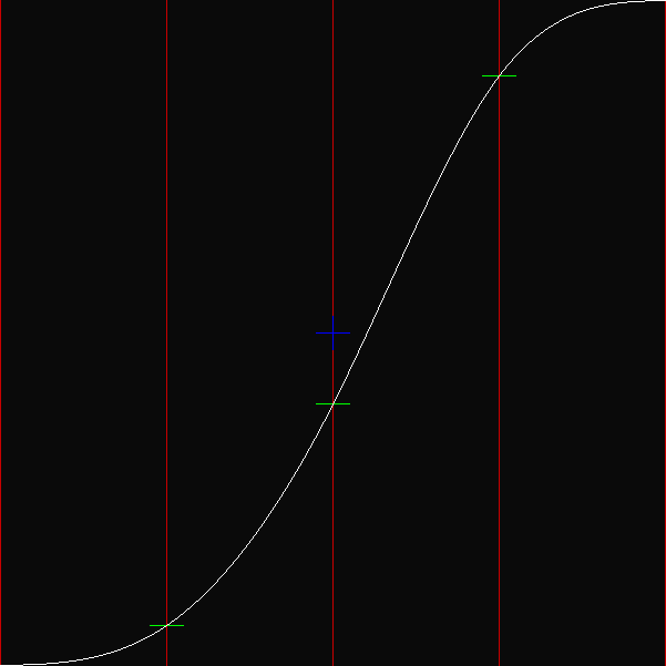
The middle "control points" are where the green horizontal line segments intersect the faint red vertical lines.
To shape the curve, move the control points along the vertical faint red lines.
To move a control point, hold the left mouse button down while moving the mouse cursor on the control point.
While this is done, the mouse cursor will change from an arrow to a hand.
You can also move the end points, but it is recommended that you don't.
To use this curve to adjust image luminances, the curve must be monotone increasing.
Nonincreasing parts of the curve will be shown in pink.
You can also avoid nonincreasing parts by setting the fourth parameter, Constrain Monotone Increasing, to True, but I find that this makes adjustments more difficult.
The seventh parameter, Control Points Preset, sets the control points to the points of the selected function before you make adjustments. If you want to make further adjustments to a previously designed curve, this parameter should be set to None.
The control points (and their number, 6th parameter) plus the 1st, 2nd, 3rd and 5th parameters generate a lookup table that is used on the pixel luminances. The dimensions of the graph are always equal to the Number of Lookup Elements (5th parameter). The curve does not generally pass exactly through the control points. To increase/decrease the vertical distances of the curve from the control points, decrease/increase, the 3rd parameter, Weights for Middle Points. The graph image can be saved and processed like any other image, but you may first have to create a floating point buffer (Control+Y). After restoring the temporarily saved image by unchecking this menu item, apply the curve with F2 or its inverse with F3. Note that your custom curve can be saved by incorporating it into an action. This operation can be painted.
Self explanatory. Color in checked queue is applied.
F2/F3 interpolates/extrapolates between the input image and a homogeneous image of the color specified in the checked queue element. By placing the median color of the image into the queue element, conventional contrast adjustment can be derived.
Sets pixel intensity values to zero.
Uses the top two queue coordinate and color entries to produce a linear variation of color.
Self explanatory in RGB space.

New with SAR 3.1! All image morphing is done with Lanczos3 interpolation! (Previous versions used bicubic.)
The image will be rotated about its center by any amount entered into the dialog box. Starting with v. 3.1, you can also shift by an arbitrary amount. The unknown portions of the rotated image will be filled with a reflection which often, especially for small angles, will provide plausible fiction. If you do not like these reflections, set the mask (press M key) before the rotation. Then, after rotation, reflected parts will be unmasked. These unmasked portions will be displayed as black, but do not directly affect the image. To make these portions actually black, press zero key.
If you load this operation into the F2 and F3 keys, pressing the F3 key will rotate and translate opposite to the amounts entered. The F2 and F3 keys will undo each others' effects, except there will be a small amount of blur/artifacts remaining from interpolation. You have the option of reducing these blur/artifacts with iterative refinement. Translation is after/before rotation for F2/F3, respectively.
Uses the checked coordinate in the Queue as the destination point. Recall that a point is entered into the Queue by left clicking on image point, followed by pressing Enter key. The source point is similarly recorded, but without pressing the Enter key. When the F2 key is pressed, the image will be translated so that the spot in the image marked by the source point is now at the destination point. The image will wrap around the canvas so that no portion of the original image is lost. The F3 key switches source and destination points and therefore can be used to undo the F2 operation.
Tips: Afterwards, fine one pixel adjustments can be made by using the Arrow keys with Ctrl key held down. When manually aligning an image in the top layer to an image in the bottom layer, it is useful to use Options>"Show Difference Between Layers," (press D key).
This operation uses the top two coordinates in queue as destination points. These points are entered by left clicking the mouse cursor followed by pressing the Enter key The source points are similarly produced but WITHOUT pressing the Enter key. The image will be translated, rotated, and resized so that the spots in the image marked as the source points are moved to the destination points by morphing the image. Similar to Rotation (see above) unknown portions of the image will be filled in with reflections and etc..
Similar to above, but uses two sets of four points as source and destination. With the Perspective Crop setting, the source points are those with the Enter key and the destination points are automatically the corners of the image.
When set and there is second layer of equal dimensions, Crop will be applied to both layers.
This allows selection of the area to be cropped by entering coordinates of the bottom left corner and dimensions of the selected area in a dialog box.
Also, this can be used as a fine adjustment to cropping with the mouse. With the right mouse button held down, moving the cursor over the image will produce a rectangle. (Paint must be off.) As the mouse is moved, the dimensions of the rectangle is displayed in the first pane of the status bar. Normally, upon releasing the right mouse button, the image is immediately cropped to that rectangle. However, if the Ctrl key is held down while the mouse button is released, there will be no immediate cropping and the rectangle will remain. Then, when Crop is used, the coordinates and dimensions of the rectangle will appear as default values in the dialog box which, then, may be edited.
Tip: Mouse crop large images by using F5 and F6 view options.
Self explanatory.
Self explanatory.
Self explanatory.

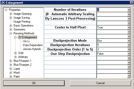
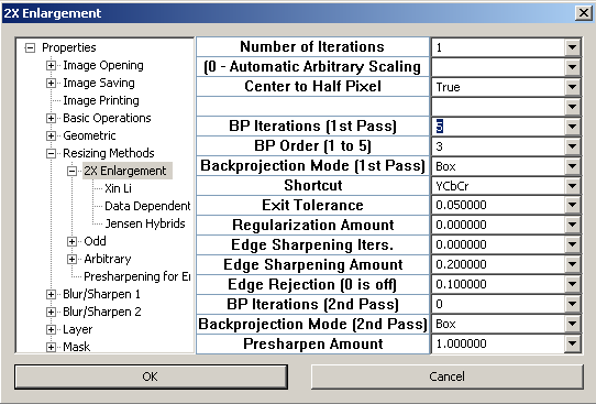
The interpolation methods, Box, Bilinear, Bicubic, Triangulation and Lanczos directly resize images to arbitrary scales or dimensions. For these, the dialog box parameter settings shown in Figure 3 must be set. However, Xin Li, Data Dependent Lanczos (DDL) and Jensen Hybrid methods directly enlarge 2X only, and with repeated iteration, 4X, 8X, 16X, 32X, etc. Also, Xin Li, DDL, and Jensen results are intrinsically 1/2 pixel off center. With the centering parameter of Fig. 2 set to False, the off center shift would accumulate with repeated iteration, i.e, 3/2, 7/2, 15/2, 31/2, etc. With the centering parameter set to True, the off center shift stays 1/2 with repeated iteration. The number of iterations and centering is set with the dialog shown in Figure 2. If the number of iterations is set to zero, the Dialog Box of Figure 3 will appear, allowing the user to resize to arbitrary dimensions using Xin Li, DDL, and Jensen Hybrids. Furthermore, centering will be exact. This is important because exact centering is necessary for making PSNR measurements on image quality. Internally, the image is resized to the next greater power of two, and then reduced to final size and shifted to center with Lanczos 3 interpolation. For example, if you resize 2.01X, internally the image is enlarged 4X and then reduced to 2.01X.
The Modified S-Spline directly magnifies only by odd integers, e.g., 3, 5, 6, etc.. As with the aforementioned 2X methods, specifying a scale factor of zero in the initial dialog will cause the Dialog Box of Figure 3 to appear, allowing arbitrary scaling.
Currently, SAR's IFS and Pseudoinverse only enlarge to integer scale factors, 1X, 2X, 3X, etc.
All interpolation methods, except Backprojection Methods, now show a progress bar in the 6th pane of the status bar. Also, pressing the Break key while the progress bar updates will terminate processing. Bug Warnings: If the running SAR program loses focus or after there has been a screensaver or monitor sleep under Windows XP, the progress bar stops displaying. This is not a crash! The Break key can still be used to stop processing. This progress bar display problem can be remedied by running SAR in XP's Win 98 compatibility mode. Another bug is that the Break key will continue to work even when SAR does not have focus.
Finally, except for IFS which automatically uses YCbCr, all interpolation methods operate in the user selected color space. It is often useful to resize using YCbCr color space instead of the default RGB. Most other color spaces are usually useless, but the option remains for experimenters.
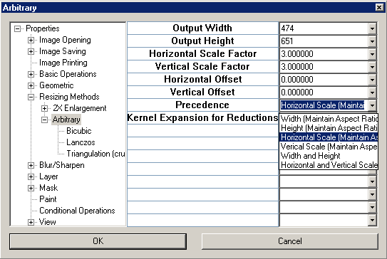
Refer to Figure 3. "Precedence" values have the following effects:
Kernel Expansion for Reductions - Only affects reductions made by Lanczos, bicubic, bilinear and Box interpolation. With this option set to False, it is appropriate to blur the image before reduction.
|
||||||||||||||||||||||||||||||||||||||||||||||||||||||||||||||||||||||||||||||||||||||||||||||||||||||||||||||||||||||||||||||||||||||||||||||||||||||||||||||||||||||||||||||||||||||||||||||

|
Normally, SAR uses floating point buffers. For image enlargement, this consumes so much RAM that the user can easily receive an "Out of Memory" message. To conserve RAM, Box, Bilinear, Bicubic, Lanczos, Triangulation, and Xin Li methods can be used directly on 24 bit data. Alternatively, File->No Floating Point Buffers On Read can be used. However, do not use these options if there is no RAM shortage because the calculations are more accurate with the floating point buffer. In Resizing Methods section of Properties Dialog Box, there is a scratch disk option which will help conserve RAM at the cost of some speed loss.
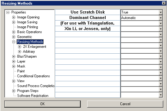
In particular, the scratch disk option is useful with the Jensen Hybrids when used without floating point buffers.
Also, called "nearest neighbor," in enlargements, it magnifies each pixel. In reductions, pixel outputs are obtained by simple averaging of pixels within nonoverlapping square areas. Enlargement results are visually unappealing, but reductions are fairly descent looking. This is the only rescaling method offered here such that upscaling by integral scale factors, followed by downscaling to original size, gives a result exactly identical to the original image. However, the backprojected offered, here, have approximately this property and, unlike Box, produce visually appealing enlargements.
Tip: This characteristic can exploited to achieve precision results during hand editing in Paint mode. First, enlarge by an integral scale factor, edit, and then shrink back to original size.
Bilinear is relatively useless for enlargements but it is sometimes useful for size reductions because it produces no halos. For sharper reductions, sharpen the input image with unsharp mask, radius = 1, before reduction. Depending on the amount of reduction but, typically, you should sharpen the input image so severely that it looks absolutely terrible before reduction.
A standard method, but rarely is the user given access to an endemic parameter, called here "Bicubic Sharpening Factor." A value of -1 results in maximum sharpening and 0 results in least sharpening. A 4x4 window of input pixels is used to calculate each output pixel.
The user selected "order" parameter controls the effective size, in pixels, of the input window used to calculate an output pixel:
As order is increased, lines and edges in the output image become less jagged, but "ringing" around edges increases. Order 3 is best for most images. Note, any order between 2 and 64 can be entered.)
Lanczos 3 is most useful for size reductions because it produces sharper results with less jagged edges than other methods offered here, however, unlike box and bilinear, it produces halos.
DDL was developed by the current author and is exclusive to SAR. DDL produces results that are similar to those produced by Dr. Xin Li's original algorithm, however, it is considerably faster. The user selects an order between 1 and 5.
This has been largely superseded by DDL. Now, the Xin Li algorithm is provided mostly for educational purposes. However, the Zhao modification of the Xin Li algorithm still shows some advantages, therefore I have changed the default settings to the Zhao modification. For Xin Li's original algorithm (actually some minor differences will remain), use the following parameter settings:
This is too slow for practical use. I have included it just to prove to academic types that it can be done, produces good results, and I thought of it first. Unless you want to consider a single pixel or the entire image as a "window," this is windowless. In the 1980s, a method for replacing sliding windows in the estimation of time varying 1D autoregressive parameters was discovered. This method produced results that were superior to that of all sliding window methods. I have simply applied this method to the estimation of NEDI parameters that vary with spatial coordinates instead of time. Roughly speaking, all of the interpolation coefficients are found at one time (technically two times) by an iterative method. Neglecting roundoff error, the method converges to a unique solution. However, starting with a DDL solution, I have found that an intermediate solution (at about 500 iterations) produces a higher PSNR.
As an option, I have combined it with SuperRez Postprocessing
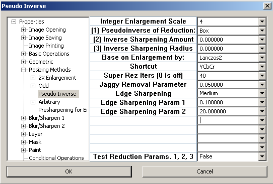
Refer to above dialog box. Pseudoinverse works only with integer scale factors. The resulting enlargement, when reduced back to original size by the method selected (1), will almost exactly match the original. The parameters of the next two lines, (2) and (3), can compensate for some sharpening or blurring. The "Inverse Sharpening Radius" is automatically scaled to the smaller image, e.g., "1" represents a radius of one pixel in the smaller image. This was to keep the settings independent of scale. Setting the last line to True will produce a reduction based on (1), (2) and (3) which can be used to match edge characteristics (halos, sharpness, etc.) of the image you want to enlarge. These settings are also used by SuperRez postprocessing. With proper settings, SuperRez will eliminate almost all edge jaggedness and halos while sharpening edges. The parameter "Based on Enlargement by" should be of slightly higher order than the method selected in (1). Otherwise, I can't tell you much because it is proprietary. Using a small crop, you should determine the settings that work best for your image by trial and error. The wrong settings will probably give bad results. I suspect that SuperRez is relatively useless for unreduced images from cameras with Bayer sensors. For Sigma cameras with Foveon sensors, I recommend the settings shown above.
There are two edge detection parameters, "Edge Detection Parameter 1" and "Edge Detection Parameter 2." Parameter 2 involves a relatively quick but sloppy test for an edge and is likely to give a "false positive" but not a "false negative." If this test is positive, a second slower but more accurate test is performed involving "Parameter 1." Increasing Parameter 2 decreases the amount of detected edges, whereas increasing Parameter 1 increases the amount of detected edges.
Smaller window sizes tend to preserve edge contours while larger windows tend to straighten edges, and/or move an edge toward its center of curvature. However, the smallest window size, 3, requires very sharp edges in the original and that is why 5 is the default. Now, in addition to odd, even window sizes are available. Often a window size of 4 is useful whereas a window size of 3 is almost never useful. Also, edges in different color channels will no longer become misaligned as with v. 1.0 Jensen.
When the mask is on, the Jensen operations will result in non-edge areas being unmasked, i.e., redrawn edges will be masked and displayed in black. This facilitates separate sharpening of textures. If this happens by accident, e.g., you accidentally pressed the M key, you may become alarmed by the blackened areas. Just press M again to remove the mask.
MBS only directly enlarges by scale factors that are odd integers. However, if the scale parameter is set to zero, then the dialog box for arbitrary rescaling will appear. The image will automatically be enlarged by the next larger odd integer and then shrunk to final size.
SAR's implementation is similar to, but far from identical to Genuine Fractals (GF). To the best of my knowledge, SAR is the only program other than GF to offer IFS interpolation. No pretense is made, GF is better than SAR's current implementation. Furthermore, unlike with GF, there is no attempt at file compression and SAR's IFS files can easily become very large.
IFS is, by far, the most complex, challenging, and intellectually interesting interpolation algorithm that I have ever encountered. Within the general IFS framework, there is almost infinite latitude for modification and improvement. And, it seems like magic to me - a rare occurrence for this old electrical engineer.
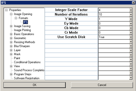
Although IFS can be accessed as a one step process from the Resize menu, it can also be accessed as a two step process from the File menu; From the File menu an image is saved as an IFS file which can be opened at any time to a desired size. In the Resize menu, IFS has been combined into single step in which internally a temporary IFS file is saved and opened. Besides allowing unregistered users of SAR to test IFS, the single step allows batch processing.
Below are the IFS dialog boxes showing default values.
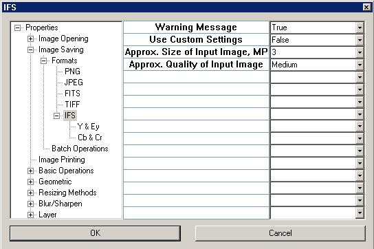

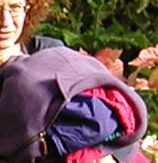
For IFS saving, there are many parameters to set, and they do have a strong influence on the results. There is one important thing to always bear in mind when using IFS; all else equal, the quality (PSNR) of the result will increase with the size of the input image. Also, all else equal, the time required for the "saving" operation will be proportional to the square of the area (megapixels) of the input image. For that reason, if you make certain settings for a large input image, IFS can take days to process. To make things easier, I have included a simplified dialog. With Use Custom Settings set to False, the custom save dialogs containing the actual IFS parameters will not appear. With the simplified dialog, the user should select the size and quality values that most closely represent the input image. The low quality setting was designed to sharpen blurry edges and obliterate noise, JPEG artifacts, and moire pattern at the expense of texture details. This setting should be considered a cosmetic effect, as it will lead to low PSNR values. I use this setting on images from my Epson 3100z digicam to obliterate moire pattern and sharpen the edges. See Figures 4 and 5.

With the possible exception of Sigma SD9 and SD10, no digital camera currently produces high quality images. However, almost any image, when sufficiently reduced in size, will produce a high quality result. Thus, researchers usually use reductions as test images for enlargement algorithms. Basically, the high quality setting is for use on reductions (Sometimes the user only has access to a reduction.) or SD9 and SD10 images.
The user can always increase the quality of the result by using a lower size setting, but processing will take much longer. For example, setting the "Approx. Size of Input Image, MP" to zero when the input image is 3.3 MP, will give a better result, but will take days to process.
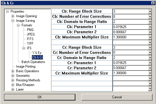
Finally, regarding custom settings, I can't explain much because that would expose proprietary information about my algorithm. Nevertheless, the user is encouraged to experiment. After making settings in the simplified dialog, the user can click on a tree branch to switch to the custom dialogs. The user can then observe the resulting changes on the actual parameters and make additional changes on the actual parameters. If these custom savings are to be saved in sar.ini, the user should then click on the IFS branch and set Use Custom Settings to True. Greyscale images can be processed faster if Cb: Range Block Size and Cr: Range Block size are set to zero in the custom settings.
In the IFS algorithm, the input image is divided into adjacent, nonoverlapping blocks called "Range Blocks" and overlapping blocks called "Domain Blocks." For a W x H image, the number of range blocks is W*H/N2, where N x N are the dimensions of the range block. The number of domain blocks is approximately (W-M)*(H-M), where M x M are the dimensions of the domain block. The user can select the range block size N and the ratio M/N = 2 or 3.
The algorithm matches every range block to a transformed domain block. The quality of the result depends on how well these matches are made. The reason that the quality of the result increases with the size of the input image is that the probability of finding good matches increases with the number of domain blocks. The IFS file records which domain block matches each range block and what transformations were made. When the IFS file opens, an output image consisting of range blocks is built out of domain blocks in an iterative process. You could say that the image is constructed out of pieces of itself starting with nothing but a set of rules contained in the IFS file. Image enlargement is accomplished by increasing the size of the range blocks in the output image, as this size is not part of the "rules."
Backprojection methods involve iterative refinement of some basic enlargement method, such that the resulting enlargement, when reduced back to original size, is almost unchanged from the input image. The greater the number of iterations, the closer the approximation to the original input image. The largest errors will be near the border of the image. Of course, this must be with respect to a particular reduction method and several methods are selectable. Backprojected enlargement has two uses. First, enlargements with backprojection have a higher PSNR ratio than without backprojection. Second, certain operations can be applied with greater precision to an image when the image is first enlarged and later shrunk back to original size. Examples of such operations include those that are manually applied or drawn. Even the quality of bicubic rotation can be improved by backprojected enlargement (use Lanczos3 mode only).
Now, the progress bar should display properly.
Referring to the above dialog box, there are three possible phases of processing. Each phase can be turned off by setting the respective number of iterations to zero.
SI has been included in SAR for educational purposes and because it has a cult following. The image is enlarged multiple times in small increments using either Bicubic or Lanczos interpolation (Lanczos 2 is practically the same as bicubic). The user selects an "approximate" scale factor, for example 1.1, after which arbitrary scale factors are selected. SAR then finds the nearest match to 1.1 such that an integer power, N, of 1.1 equals the final scale. The image is then automatically enlarged N times.
Produces results similar to QImage's "Pyramid." It is an application of the "Step Interpolation" to the triangulation method.
This is a special type of sharpening which, when used properly, will help produce an enlargement with a higher Peak Signal to Noise Ratio (PSNR) at the expense of some slight haloing. It uses a file, Kernels, that is included in sar.zip and should be installed in the same directory as sar.exe. It assumes that the image that you are trying to enlarge was produced by a reduction method, so you must enter that method (Box, Bilinear, Bicubic, Lanczos2, Lanczos3) as a parameter along with an approximate integer magnification (2 to 9). For unreduced images, you will have to find the best settings by trial and error. Not for use with IFS, LAD, or any Backprojection method (Backprojection methods now have their own version of this included as an option.) A more technical explanation follows.
For purposes of magnification of natural images, the best image model is one in which the input image is produced by the convolution of a larger image, of target size, with some smoothing kernel, followed by decimation (subsampling). This model is appropriate because all light sensors average light intensity over their surface areas. Thus, the output of a sensor does not represent the light intensity at the center of the sensor. This model accommodates other sources of blur, but the sensor source is the only one common to all natural images. Also, typically, size reduced images are produced by convolution with a smoothing kernel followed by decimation. Such images, although possibly not natural, are also accommodated by this model. Enlargements made by strict interpolation methods are intrinsically blurry because they represent approximations to the stage in the model before decimation but after convolution. Enlargement methods which use strict interpolation provide a quasi-inverse (seems like a reversal) to decimation only. In image magnification, one should seek quasi-inversion to both convolution and decimation combined. However, it is possible to perform a special type of linear sharpening to the input image that provides an estimate of a purely decimated "larger" image without convolution with a smoothing kernel. In terms of image light sensors, a presharpened pixel represents an approximation to the output of a hypothetical smaller sensor positioned at the center of the actual sensor. After such presharpening, enlargement made by almost any strict interpolation method will more closely approximate (higher PSNR) the modeled "larger" image.
SAR's proprietary presharpening method is loosely based on this paper:
http://www.ornl.gov/sci/ismv/pdfs/publications/Price-SensorOptimalImageInterpolation.pdf
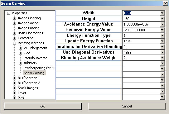
The following is optional.
By using Resize>Set F2/F3 to Draw Avoidance/Removal Regions, you can use the right/left mouse buttons to draw Avoidance/Removal regions in red/green.
You must select this from the menu for each seam carving because a temporary copy of the original is saved for seam carving.
Removal will not work for enlargements.
Don't forget to change the mouse curser by pressing P.
The width and height must be between half and twice that of the original.
However, because the quality decreases substantially for increases more than 50%, it is recommended that such size increases be done in stages with derivative blending between stages.
Energy Function Mode Types:
0 - Sum of Absolute values of derivatives in Y channel of YCbCr color space.
1 - Sum of Absolute values of derivatives in all channels of RGB color space.
2 - Square root of sum of squared values of derivatives in Y channel of YCbCr color space.
3 - Square root of sum of squared values of derivatives in all channels of RGB color space.
4 - Sum of squared values of derivatives in Y channel of YCbCr color space.
5 - Sum of squared values of derivatives in all channels of RGB color space.
6 - Sum of Absolute values of derivatives in Y channel of YCbCr2 color space.
7 - Sum of Absolute values of derivatives in all channels of log RGB color space.
8 - Square root of sum of squared values of derivatives in Y channel of YCbCr2 color space.
9 - Square root of sum of squared values of derivatives in all channels of log RGB color space.
10 - Sum of squared values of derivatives in Y channel of YCbCr2 color space.
11 - Sum of squared values of derivatives in all channels of log RGB color space.
Usually, the odd modes will produce better results but take more time than the even modes. More than other modes, modes 10 and 11 produces seams that tend to avoid passing through high contrast edges.
Update Energy Function - Apparently, in the original paper by Avidan and Shamir, the energy function was not updated between seam removals. Doing so (recommended) improves results at the cost of a small loss of speed.
Iterations for Derivative Blending ("Gradient Domain Seam Removal" or "Poisson Editing") - Zero is off. Usually, 100 iterations is enough. This reduces the severity of two kinds of artifacts:
1. Kinks in edges, ridges and lines.
2. Abrupt change of luminances in areas with previously slowly changing luminances.
Also, textures often look better with derivative blending.
Blending Avoidance Weight - Setting this to a sufficiently large value prevents derivative blending from changing avoidance regions. Although rarely needed for size reductions, it is often needed for size increases.
Example input image:


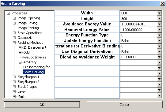
Parameter Settings for following result:
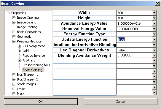

Parameter Settings for following result:

Adding Avoidance (red) and Removal (green) Regions for following result:
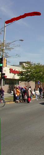

Using the immediately preceding image as input with these avoidance regions,


Same as "Average" with radius = 1, but not conditional with mask and cannot be painted, i.e. you can select color channels only. Repeated application approximates a Gaussian blur with variance 2/3 N, where N is the number of iterations.
Not conditional with mask and cannot be painted.
This operation simulates an unfocused camera lens. The user selects the Radius parameter to control the amount of blur. For variable lens blur, see Gradient Lens Blur. This operation can be painted and is conditional on both mask and color channel selection. Normally, only the result is masked; however, with the "Masked Input" parameter set to "True," masked areas will not be used as input. For example, suppose you have an image of stars in the night sky and you want to remove noise in the surrounding sky. To do this, mask the stars and use Average with "Masked Input" set to "True" to blur the noise. If this parameter was set to "False," the bright color of the stars would diffuse into the surrounding areas. Experimental results suggest that this is best used with the Gamma 2.2 color space.
Multiple iterations of this filter no longer simulate lens blur. Instead, the result (with at least 3 iterations) will be a close approximation to a Gaussian blur. However, unlike the Gaussian Blur filter provided in SAR, this can be masked and painted.
This simulates blur caused by an object moving at constant velocity. The user selects the distance in pixels and angle in degrees. Again, experimental results suggest that this is best used with the Gamma 2.2 color space.
Speed improvement with version 3.1!
Similar to Average, but median replaces average.
Median filtering is useful for removing small spots, such as stars, hot pixels, and impulsive noise.
For regular median, non-integer radii are rounded to nearest integer greater than one.
New with version 3.0
Gaussian Weighted Median allows non-integer radii (standard deviation).
Radii between 0.6 and 1 are especially useful for removing speckled noise.
Similar to Average, but wmmr replaces average. Actually, there are several types of wmmr and this is the "median" type. Removes texture details while sharpening edges.
For noise removal, I recommend that the "Window Size" (WS) be about the same size as the blotches of noise. Then use the minimum "Intensity Spread Factor" that removes the noise. Usually, this will be between 2.5 and 10. More than one iteration may be needed. If this produces posterization, the posterization can be reduced by additionally applying a few iterations with a small WS, e.g., 1, and larger IFS, e.g., 30.
This can also be used for various types of edge enhancement, such as removal of halos and sharpening. Also, edges are easier to detect after texture has been removed with the bilateral filter.
This is possibly the best noise reduction algorithm available today. Unfortunately, it is probably the slowest. As such, it is only practical for use on very small images. Also, there is considerable tradeoff between quality and speed with respect to the parameter settings. For maximum quality, the Search Radius should be set to half the maximum image dimension. Doing this, will cause the operation to practically take forever.
This causes curved edges to move toward the center of curvature. Small spots will become smaller faster than large spots. Useful for straightening jagged edges and lines, it is my experience that this is best applied to selected areas as a painted operation. It can also be used to remove impulsive noise, but, for this purpose, I see no advantage over median filtering.
The "Modulus" and "Offset" parameters are for experimental use in conjunction with removing jaggies from enlarged images. Under some circumstance, an enlarged image will contain some pixels that are unaltered from the original image. These pixels will be located at the intersection of every Mth row and column of pixels, starting with the Nth row and column. By setting Modulus = M, and Offset = N, these pixels are excluded from isophote smoothing, i.e., these pixels remain unchanged. Some people have claimed improved results, but I don't see it. If you are not experimenting with this, these parameters should be set to zero.
The "Modes" -1 and 1 refer to two different ways of implementing the algorithm. Since I noticed a very subtle difference in results, I included both. Mode 0 alternates between the two at each iteration.
Using "Average" mode and with "Sharpening Threshold" as the only threshold (other thresholds set to zero), this is equivalent to conventional unsharp mask. When the absolute value of the difference between pixel intensity values of a blurred and unaltered image is less than the threshold, the aforementioned difference is subtracted from original, thereby selectively sharpening areas of low sharpness.
The unconventional "Blur Threshold" and "NoOp Threshold" are thresholds below which the image is, respectively, blurred and unaltered. These can allow sharpening without enhancing noise. These thresholds are tested in order:
1. Blur
2. NoOp
3. Sharpening
All thresholds are expressed as a fraction of the color space range.
This has been changed considerably with version 2.03. The operation can now be masked and/or painted. It will sharpen, smooth, align edges, and remove halos. One disadvantage of Jensen is that it has a tendency to round corners. Curved edges tend to be moved toward the center of curvature.
Credit goes to Donald Graft (aka neuron2) for the XSharpen algorithm. This filter can be used to sharpen severely blurred edges such as those found in enlargements, but the results tend to be slightly ragged. The one advantage that this has over Jensen is that it does not round corners. This can be followed by Jensen Edge Enhancement to smooth edges. This can be masked and/or painted.
This algorithm was developed by Dr. David Tschumperl� for his Ph.D. Thesis. The version presented in SAR's Blur/Sharpen menu is particularly useful for removing certain types of noise. Another version is presented in SAR's Paint menu for inpainting. I have made several modifications.
The amount of effect is controlled by both the number of iterations and the step size. There are two step size parameters, one for blur and one for edge contiguity. In the original algorithm, these were equal except, for inpainting, blur step size was zero. Larger step sizes allow fewer iterations, however, unwanted artifacts are likely to appear in homogeneous regions. I have also provided a "Blur Parameter" and "Edge Parameter" to help control these artifacts. Higher values tend to reduce the aforementioned artifacts. In the original algorithm, these were both set equal to one.
The "Mode" parameter selects one of two ways that discrete derivatives are calculated. Mode 1 is the original used by Dr. Tschumperl�, whereas Mode 2 tends to produce sharper diagonal edges.
In the original algorithm, certain quantities were recalculated at every iteration. I found that recalculating these quantities only on every 10th or 100th iteration results in a substantial savings in time with little loss of quality. The user controls this with the "Recalculation Interval" parameter. If the Recalculation Interval is set to one, recalculation is performed as in the original algorithm.
This is intended for use with RGB color space, but the user has the option to experiment with other color spaces. This operation cannot be separately applied to individual color channels, but it can be masked and/or painted.
This is basically an edge sharpening filter. Internally, the algorithm is similar to the above Tschumperle Regularization which the user should see for an explanation of Mode and Step Size parameters. With the "Standard Deviation 2" parameter set equal to zero, it is a standard shock filter. Dr. Joachim Weickert modified it for "enhancement of coherent flow-like structures" such as fingerprints. It can also be used to create artistic effects. Dr. Weickert's exact version is not available here because he calculated derivatives differently (namely with Sobel masks).
This is for removal of semi-transparent repetitive patterns. The user may select one of two Pattern Type presets, crosshatch and honeycomb. When crosshatch or honeycomb are selected, the Number of Points and the Index Offsets are automatically calculated. Then the user need only enter Smoothing Function and Radius or Period of Repetition. Custom patterns can also be accommodated by manually entering Number of Points and Index Offsets, but further instruction on custom patterns will not be given.
Consider this example of an image with a honeycomb pattern:

The five steps to remove the pattern while retaining detail are:

In the example, I used the regular median filter (Blur/Sharpen>Median) with a radius of 4. Tip: For patterns that are faint and only visible in otherwise homogeneous areas, it might be better to use bilateral filter or Tschumperle regularization to obtain a "crude" start.
Observe that the pattern is of nonstationary intensity.
Observe that the process is less effective near the borders.
The image at this stage can be used as the final result or a faint remaining pattern can be further removed. You can remove a faint pattern using bilateral filter or Tschumperle regularization, spot retouch or globally, and repeat the process, substituting this for the intermediate result of step 1. The details in step 2. will be more faint and therefore more easily removed by a single repetition of periodic smoothing.
Finally, some adjustment of contrast and brightness is advisable.
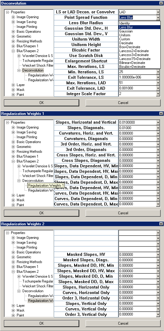
This is for deblurring or enlargement of small images. SAR offers two types with Tikhonov style regularization, Least Squares (LS) and Least Absolute Deviations (LAD). Referring to the first parameter of the above dialog boxes, the user can select "LAD", "LS", or "Convolve." The "LAD" and "LS" operations are quasi-inverses to the "Convolve" operation. The type of "Convolve" operation is selected via the second parameter in the dialog box. Any selection with "decimate" in it will produce a reduced size image with "Convolve" and an enlarged image with "LAD" of "LS."
Both LAD and LS deconvolutions are calculated iteratively. LS typically requires 25-500 iterations. LAD uses two levels of iteration, one nested inside the other. The inner level of an LAD calculation is an LS calculation. The outer level typically involves 15-50 iterations. The progress of calculation is reported in the status bar. The fourth pane reports the color channel, X, Y, or Z, being calculated. The fifth pane reports the number of iterations to find an LS result.
The sixth pane reports the following three quantities separated by commas:
1. The number of LAD iterations completed.
2. A quantity to be minimized for LAD, more specifically, the actual L1 norm of errors.
3. A quantity that converges to zero and is used as a stopping criterion for LAD (stops when less than LAD Exit Tolerance).
The accuracy of LS calculations increases with the number of iterations. To obtain a visually accurate LAD result, the inner LS calculations must be sufficiently accurate. Usually, "sufficiently accurate" can be surmised through trial and error variation of the number of inner LS iterations while inspecting the final L1 norm of errors over the trials.
Tikhonov regularization is a method for imposing smoothness constraints on LS solutions. Here, we impose similar constraints on LAD solutions and call them "Tikhonov style" regularization. The smoothness of the results can be increased by increasing the regularization weights in the above dialog boxes. Tikhonov regularization can be used with the identity operation to produce artistic effects or, in the case of LAD, removal of impulsive noise. The sole advantage of LAD over LS resides in way that different smoothness constraints behave. With LS, there are little differences between the effects of different smoothness constrains, whereas, with LAD, these differences are pronounced. It is instructive to examine the effects of different smoothness constraints with the identity operation in the following images:

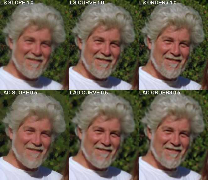
Observe that the LAD slope regularization is very different from the rest in that it produces sharp edges and areas of constant color. Although not visible in the above examples, LAD slope regularization excels at suppressing ringing and halo artifacts. Also, LAD regularization will remove impulsive noise better than median filtering:
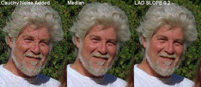
The peak signal to noise ratios in the green channels of the above three images are, left to right, 20.2, 28.8 and 30.0.
A convolution kernel, called "Point Spread Function" (PSF), must be assumed. Various types of PSFs correspond to different physical causes of blur. Each type of PSF has parameters that must be set by trial and error. Because of the slowness of this operation, it is recommended that trial and error work begin on a small crop of about 50x50 pixels. The "Lens Blur" PSF is for blur caused by an unfocused camera lens. The "Gaussian" PSF is for blur caused by atmospheric turbulence, as is often the case for astronomical images from telescopes. The "Uniform" PSF, with Width/Height set to 1 can be used for blur caused by constant motion in vertical/horizontal directions. For deblur of motion in directions other than horizontal or vertical, the image can first be rotated so the direction of motion is horizontal or vertical. After deblurring, the image can be rotated back to its original position. For these purposes, Backprojection can be used for high quality rotation.
Under ideal conditions, deconvolution can produce amazing results. Ideal conditions include:
This was artificially produced with a lens blur of radius 10:
This is the result of LAD deconvolution of the above image:

Pretty impressive, huh? Unfortunately, in practice, nonideal conditions lead to much less impressive results. The following image was made with an unfocused digicam:
This is the result of LAD deconvolution:
I do not know which nonideal condition is most damaging in this example, but I suspect it is a nonlinear transformation of luminances within the camera.

The enlargement operations here should be viewed as quasi-inverses of size reduction processes. Unlike the previous lens blur example, near ideal conditions are more commonly encountered in practice. Often people make a reduction of an image and then lose the original. In those cases where the reduction method was one of those selectable from listed Point Spread Functions (+ Decimate), the resulting LAD enlargement will have superior fidelity to the original. It should be noted that the Backprojection methods discussed elsewhere comprise cruder methods of this sort. Under less ideal conditions, Backprojection methods may provide adequate results more quickly.
To enable this you will have to first create or load a noise profile. To create a noise profile, you will have to find an image that is typical of those you want to process, but with a homogeneous area such as blue sky. Within this homogeneous area, form a rectangle, large as possible, by dragging the mouse cursor with right button down. Hold down the Control key down while releasing the right mouse button, or you will crop the image!!! The current color space will become part of the noise profile. You may change the color space at this time. Then click Create Noise Profile. A dialog box will appear that allows entry of numbers separated by commas. The first of four numbers represents the number of frequency levels. Large blotches of noise will require more levels and therefore will take more processing time. The next three numbers correspond to degrees of compensatory sharpening (0, 1, or 2) for the three color channels. After clicking OK, three more dialog boxes will appear, each corresponding to a different color channel. The numbers in these dialogs are wavelet shrinkage parameters found by analysis of the selected rectangular region. Normally, these do not need editing, but you can at this time. These parameters correspond to different frequency levels ranging from highest to lowest, left to right, respectively. Increasing these parameters decreases noise and image details. You can conveniently multiply or divide these numbers by literally inserting "*" or "/" followed by a multiplier. After creating a profile, you may save it with Save Noise Profile (or not).
Once a profile is created, you can use Fast Noise Removal on as many images as desired. Processing a 3.3 MP image typically takes 2 seconds.
Since the color space is an important part of the noise profile, you should experiment with different color spaces. For each additional color space, you need to create a new profile, but it will usually be unnecessary to form a new rectangle, even though the old rectangle is no longer visible. In particular, I find YCbCr particularly useful. I multiply the wavelet shrinkage parameters for the "chroma channels" Cb and Cr channels by 4.
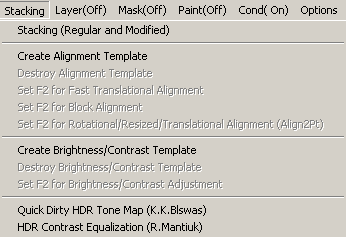
Combines multiple pictures of identical or slightly changing scenes from files selected with a file opening dialog box. In this dialog box, you make multiple file selections the same way you would with Windows Explorer. During processing, the number of images is counted in the fifth pane of the status bar.
Attention! Images must be in alignment. If not in alignment, the images must be digitally aligned before stacking. See, How to Align Images from Hand Held Camera, below.
SAR has six modes:
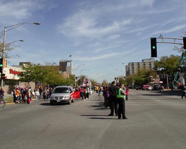
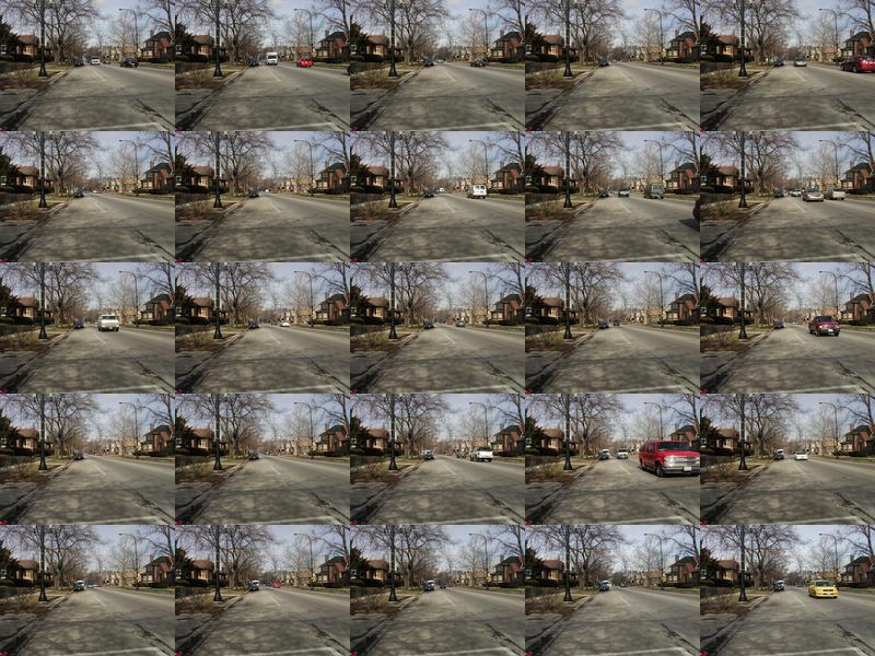
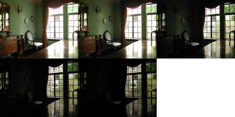
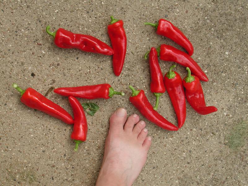
The following shows 25 exposures of a street with passing cars.
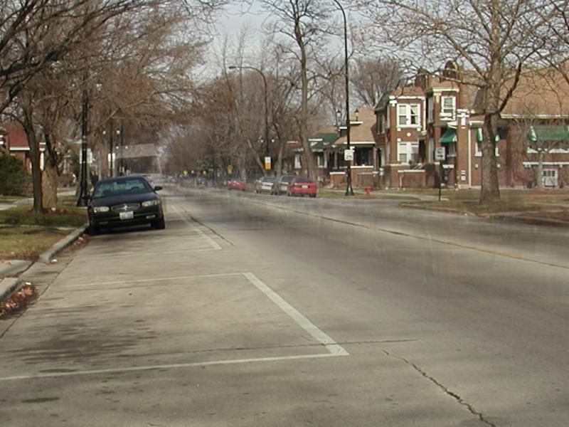
The following is the cropped result of regular Average stacking on those images.
Observe that ghost-like images of the passing cars, especially along the center of the street.
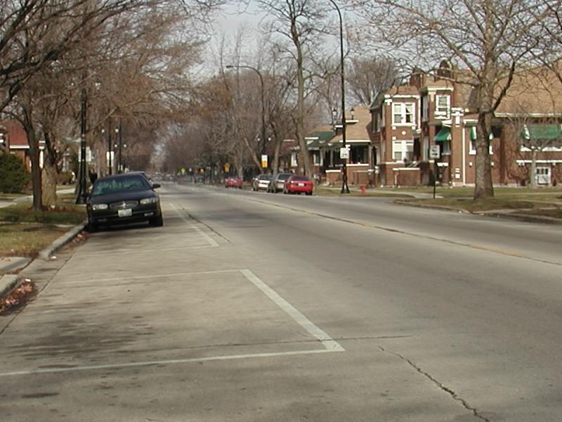
The following is the cropped result of Multivariate Median 2 stacking on those images.
Observe that almost all traces of the passing cars were removed.
http://www.janrik.net/ptools/ExtendedFocusPano12/index.html
http://helicon.com.ua/pages/focus_samples.html
Some of these images first need to be aligned (see below). I think you will find that SAR's Extended DOF outperforms the competition with respect to both quality and speed.
This makes a greyscale template from the image to which other images will be aligned. The alignment operations are disabled until this template is created.
Because the alignment template uses large amounts of RAM, it should be destroyed after use.
Typically, you will use a tripod and interval timer to take pictures for stacking. Even so, wind or manual camera adjustments may cause small shifts between images. This operation is mainly for aligning such images prior to stacking. To enable this, you must first create a template from an image, after which, pressing F2 will quickly align a similar image to the one used in creating the template. Alignment may fail if the image is misaligned by more than 1/3 the minimum dimension of the image. During alignment, portions of an image extending beyond its border will be wrapped around to the opposite side. After finishing all alignments, you should destroy the template to free RAM. If used in Batch processing, there is a setting in the Batch dialog box that automatically destroys the template at the end of Batch processing. It typically takes 1 second to align a 3.3 MP image.
Attention! This operation is usually necessary for accurate alignment of images from a hand held camera! There are two versions of this operation, one found under Stacking, another found under Layers. Both share the same parameter settings. The difference between the two is that Stacking version aligns images to a greyscale "alignment template" whereas the Layers version aligns the top layer to bottom layer using all color channels. The Stacking version is about three times faster but slightly less accurate. This operation first finds shifts in small non-overlapping blocks and then interpolates these shifts to align images. Although only shifts are involved, this alignment procedure can compensate for many different kinds of distortions, including small rotations. It is important to set the Search Radius greater than the maximum misalignment in pixels. However, the greater the search radius, the slower the operation. Typically, images previously aligned by Set F2 for Rotational/Resized/Translational Alignment (below) will be within 3 pixels, the default search radius for Block Alignment. For Block Alignment, it is important that the alignment template not contain passing objects. For Rotational/Resized/Translational Alignment, passing objects are much less deleterious. The nominal accuracy of SAR's Block Alignment is 0.0625 pixels.
This is for aligning images taken with a hand held camera. Although not unreasonably slow (about 1 minute for a 3.3 mp image), this operation is not perfectly reliable therefore images should be inspected after using this operation for accurate alignment. Similar to Geom>Arbitrary Rotation, unknown portions of the image will be filled with reflections.
This operation is used to compensate for changes in lighting conditions, such as those caused by passing clouds, prior to alignment. Otherwise, if the exposures vary greatly, the images may fail to align. Similar to the above alignment operation, you must first create a template.
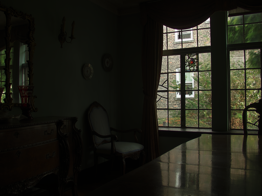
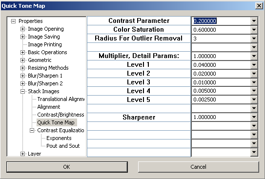
K.K.Biswas and S.Pattanaik, "A Simple Tone Mapping Operator for High Dynamic Range Images," School or Computer Science, University of Central Florida This can be used on normal low dynamic range images by setting the Contrast Parameter equal to zero.
This is the result of processing the previously stacked image:
with these settings:
Although not obvious here, the method is "dirty" because it often produces visible halos.
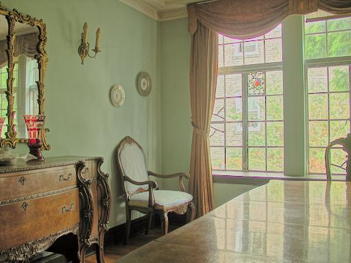
This is the result of processing the previously stacked image:

with these settings:

Typically, a CE result will benefit from post sharpening which has not been been done here.
CE involves an iterative process that can take up to 1500 iterations to become visually stable. One SAR modification is to use a QDTM result as the starting point for iteration. In some cases, this produces a visually useful result in as little as 10 iterations, usually, by eliminating halos from QDTM. Thus, the dialog box for QDTM will appear before the one for CE. Two parameters, Color Saturation and Radius for Outlier Removal, are shared by both methods. The Radius for Outlier Removal is explained under Basic>Scale and Shift to [0,255].
I am unsatisifed with SAR's current Contrast Equalization, so it is likely to change in the near future and that is a reason why I am not fully explaining the settings. Sorry, for the inconvenience.
There are advantages, other than convenience, to stacking digitally aligned images from a hand held camera instead of from a camera with tripod. After digital alignment of slightly misaligned images from a hand held camera, JPEG artifacts, demosaicing and other sensor based anomalies will occupy random positions and therefore be reduced as noise by stacking.
You should align an image set in at least two stages, first, by using one image from the set as a template, and, second, by using the result of multivariate median stacking of the first aligned set as a template. It is done this way because noise and passing objects in the first alignment template will contribute to inaccuracies in the first set of aligned images. Multivariate median stacking will reduce noise and passing objects from the template used in the second stage.
I can't anticipate all contingencies, so, please, use common sense; I want this to work for you.
1. Try to select a good image from the set to be aligned. You can optionally make rotational adjustments on this. Create an alignment template from this image.
2. If the exposure of every image in the set is visually similar, skip step 2 and go to step 3. Otherwise, e.g., there was variable shade from passing clouds, create a Brightness/Contrast template and use Set F2 for Brightness/Contrast and batch process so the images have similar brightness and contrast. This is necessary because the multivariate median stacking used in step 4. does not perform well with variable exposures.
3. Batch process the images with Rotational/Resized/Translational Alignment.
4. Stack the aligned images using Multivariate Median.
5. Create a new alignment template using the multivariate median stack result. This is done to remove passing objects from an alignment template so that the passing objects won't interfere with Block Alignment.
6. Starting with either the original set or the brightness/contrast adjusted set, use Rotational/Resized/Translational Alignment followed by Block Alignment. You can either do this as two batch processings, or you can combine the two operations into one action and apply in one batch processing.
7. Although rarely necessary, for extra accuracy, you can repeat starting with step 4.
8. Tips: Use copies of your original files so you don't lose them by accident. A good file format to use for batch processing output is 16 bit/channel PNG. After batch processings, it is often useful to inspect intermediate results with Sequential Load (F9).
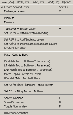
This toggles creation and destruction of a second layer. No more than two layers can be created. These layers consume a lot of RAM.
Creates a second layer with the same dimensions as the first. (The new layer will contain a black image.) However, the two layers will not necessarily remain the same size because, afterward, the size of each individual layer can be independently changed. Bear that in mind, because most operations that simultaneously involve both layers are disabled when the dimensions do not match. The old layer and newly created layer are respectively designated as "Layer 1" and "Layer 2." Either layer will be called the "top layer" when it is normally visible and either layer will be called the "bottom layer" when it is normally invisible. Operations involving only one layer are applied to the top layer. The top layer is indicated in the fourth pane of the status bar. Also, the existence of a second layer is indicated on the menu bar as "Layer( On)."
When a second layer is destroyed, it is always Layer 2 (even if Layer 2 is on top).
Exchanges the top and bottom layers. If there is only layer, a second layer will be created.
With Conditional Operations checked ("Cond( On)" in menu bar), and provided that top and bottom layers are the same dimensions, this operation can be painted and this is conditional on color channel selection and masking. With Conditional Operations unchecked, all channels and mask of bottom layer will be copied to the top layer.
This is a sophisticated modification of the above which blends the boundary and, to a lesser extent, the interior of a region transferred from the bottom to the top layer. It is most useful for cloning textures, e.g., skin textures, removing tatoos, etc. This operation is always applied to all color channels and there must be a mask with an unmasked region OR the operation must be painted. Of course, painting can be used in combination with a mask. The derivative blending is an iterative process and the result depends on both the number of iterations and the starting point.
Example:
Original:
Cloned without derivative blending::
Cloned with derivative blending::
Pixel values at corresponding coordinates throughout the images are added/subtracted.
Tip: This can be used to incrementally sharpen images. Exchange layers and duplicate image in bottom layer (=). Then blur the image and subtract the bottom layer. Exchange layers again and use F3 to sharpen image.
The F2 "Interpolate" operation is represented by the following equation:
(1-C)*(top image) + C*(bottom image)
where C is the parameter entered in the dialog box. In other words, the result is a weighted average of the two images. The F3 "Extrapolate" operation is the inverse to this weighted average.
Tip: This, also, can be used to incrementally sharpen images. Exchange layers and duplicate the bottom layer (=). Then blur the image and exchange layers again. Set F3 to Extrapolate and use F3 to sharpen image.
Similar to Lens Blur except variable radii values are given by pixel intensity values in bottom layer. See Gradient and Lens Blur.
If the top and bottom layers are of different dimensions, this will match the sizes of the layers. The images contained in those layers will be retained and positioned with coincident lower left corners.
Tip: To reposition images on layers, use "One Point Registration" and/or Ctrl + arrow keys.
This is for use on similar images, for example, as a preconditioner to stacking. The top and bottom layer images must be of the same scene and aligned. This operation matches, in the least squares sense, the brightness and contrast of the image in the top layer to that in the bottom layer.
Similar to above, but too difficult to explain. Feel free to experiment.
This works best in log RGB or log CMY color spaces. Again, top and bottom layer images must be of the same scene and aligned. Roughly speaking, this operation matches portions of the histogram of the top layer to portions in the bottom layer.
This is used to tile images like this:
First, you must create a blank canvas and put it on the bottom layer. You can do this Geom>Create Blank Image, followed by pressing the X key. Then, load a smaller image to be tiled. Next, select Set F2 for Tiling Top into Bottom from the menu. This initializes the operation so that, the first time F2 is pressed, column and row counters are initialized. Also, the first time you press F2, the top image will be transferred to the upper left corner of the bottom layer, after which the bottom layer will be copied to the top. Repeatedly loading new images and pressing F2 will continue the tiling from left to right and top to bottom. If you need to start a new tiling, don't forget to reinitialize again by clicking Layer>Set F2 for Tiling Top into Bottom in the menu. This operation can be combined with image size reduction using Prog>Record Program and/or used with File>Batch Operation, but don't forget to reinitialize
Displays a weighted average of top and bottom layers (RGB only). This is useful for manually aligning dissimilar images via One Point Registration and Ctrl (or Shift) + Arrows keys.
Displays absolute difference of top and bottom layers (RGB only). This is useful for manually aligning similar images via Ctrl (or Shift) + Arrows keys.
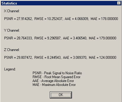
This feature is enabled when equal sized images are in the top and bottom layers. It reports statistics on the differences between the two images. This feature can be used to compare the quality of results from different enlargement methods. First, a large original is reduced, usually using box interpolation. Then this reduction is enlarged to original size by the method being tested. The statistics on the differences between the enlargement and original serve as objective criteria for determining which enlargement method is best. The most commonly used measurement is Peak Signal to Noise Ratio (PSNR) (larger is better). Alternatively, one can use Root Mean Squared Error (RMSE) or Average Absolute Error (AAE) (smaller is better). AAE is less sensitive than RMSE to a a few large errors. However, these measurements do not tell the whole story. All else equal here, structured errors are worse than unstructured errors, but, to my knowledge, nobody has quantified this yet.
It is important to remember that scaling must be virtually exact with no shifts. I mention this because the interpolation methods of other vendors often do not meet these criteria. With suitable parameter settings, all of SAR's interpolation methods meet these criteria.

Most of the following mask operations will create a mask when one doesn't already exist. By default, unmasked regions will be displayed in black. This "black" is not saved to file or printed, it merely shows you which part of the image is unmasked and masked: the black areas are unmasked and non-black areas are masked when Mask->Show Unmasked Area is checked and visa-versa when Mask->Show Masked Area is checked. Press S key to toggle this display feature. Also, there are other mask display options. In particular, you can see a bottom layer through an unmasked region of the mask on the top layer by using Shift+S.
When a new image file is opened (except for FDIB files), if the new image has the same dimensions as the image that it replaces, the mask of the old image will be retained. If the new image has different dimensions than the old, the old mask is destroyed. FDIB files store the mask with the image.
Toggles mask creation and destruction.
Creates a one bit depth mask for the top layer. Upon creation, all mask bits are zero (all pixels masked). The mask can only be saved with *.fdib image files. The existence of a mask is indicated on the menu bar as "Mask( On)."
Sets F2/F3 keys to set mask bits to 1/0. This operation can be painted.
This operation is conditional upon color channel selection. Also, some color spaces will show advantages over others.
This operation unmasks edge areas of the image. Unmasked areas will be displayed in black. F2/F3 increments/decrements a tolerance parameter such that F2 increases the unmasked areas and F3 decreases the masked areas. When recording actions, individual key pressings are not recorded, only the final tolerance.
Masked areas become unmasked and vice versa.
Sets unmasked areas in the top layer to the union of unmasked areas in the top and bottom layer masks.
Sets unmasked areas in the top layer to the intersection of unmasked areas in the top and bottom layer masks.
Extends the edge of an unmasked area by one pixel.
Draws horizontal and/or vertical bars. This involves a departure from SAR's convention of having a coordinate origin at the lower left corner of an image. Here, the origin is the upper left corner because 8x8 JPEG blocks start there and this mask feature is useful for blurring the border between JPEG blocks.
Displays unmasked areas in black.
Displays masked areas in black.
Displays bottom image through unmasked areas of top image. Useful for positioning portions of the bottom image before transferring to top image.
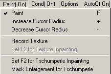
When checked, the cursor should change shape and become a circle with a dot in the center. The diameter of the circle is controllable with the numerical keypad + and - keys. There is a bug under Windows ME/98 such that the cursor does not change. The size and appearance of the cursor can also be controlled from the Properties Dialog which will appear when the Ctrl key is held down while clicking Paint.
By holding down the right mouse button and dragging the cursor, most F2 programmed operations can be painted. The swept area will temporarily appear black and the operation is applied upon releasing the button. Similarly, the middle mouse button paints F3 programmed operations. With "Cond(Off)" painting is unaffected by a mask. With "Cond( On)" painting is applied only to the union of unmasked regions with the area swept by the paint cursor. If operations that can be painted are combined in an action, the action can be painted.
1. Select an appropriate color space, usually YCbCr.
2. Select a rectangular textured area as shown, for example, in this figure:
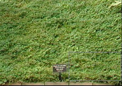
This is done by holding the right mouse button down and dragging the arrow cursor as in crop, but hold Control key down when releasing mouse button to prevent crop.
3. Then click on Record Texture which should now be enabled.
4. Click Set F2 for Texture Inpainting.
5. The texture can now be masked and or painted. The sign in the figure below was painted over.

6. When you are done with this operation, click Destroy Texture (formerly Record Texture) to release memory used for texture recording.
The textures are drawn in a diagonal direction from top right toward bottom left and, as such, tend to be congruent with areas adjacent to mask edges facing the top right and incongruent with other areas. Also, lines within a texture and approximately parallel to the drawing direction are well preserved. The drawn textures are based on pseudorandom numbers and are, therefore, different every time drawn. Thus, it is recommended that areas be painted several times until a result that is pleasing to the eye is achieved.
I have found this useful for accurately simulating digicam noise or film grain in otherwise noiseless digital images. The procedure follows.
A. Use logCMY color space.
B. Find a small, e.g., 100x100, homogeneous area with noise or grain to be simulated and crop it. (By "homogeneous," I mean homogeneous except for the noise or grain.)
C. Duplicate this to a second layer.
D. Blur out the noise in one layer, e.g., with 1000 iterations of Fast 3x3 Average, and then subtract this from the unblurred layer. (With logCMY color space, the result will appear mostly white but with noise or grain.)
E. Use this result to Record Texture.
F. Destroy the second layer and load the image to which you want to add noise. (You should still be logCMY space.)
G. Create a second layer by pressing X. (This will appear white.)H. Set F2 for texture inpainting and press F2. You now have a simulated transparency, almost clear except for noise or grain.
F. Add the two layers.
The result will be like a print made from two stacked negatives, one without noise or grain and the other clear except for noise or grain.
This fills unmasked areas so that outside edges connect. In the example below, the black, unmasked areas are inpainted.

This is done in two stages which can be performed separately or together. The first stage is turned off by setting Initialize to False and the second stage is turned off by setting Iterations to zero. The first stage serves as a quick initial approximation and is simply a blurring of masked pixels into the unmasked regions. In the example, the result of the first stage is shown in middle. The second stage is the actual Tschumperle inpainting. The result of Tschumperle inpainting is shown at the bottom of the example image. The wider the gap to be filled, the more iterations are necessary. With the first stage turned off, the Tschumperle inpainting can be applied in cumulative steps by pressing the F2 key repeatedly until the widest gap is filled.
The Dominant Channel parameter provides some modifications to the original algorithm. In the original algorithm, certain calculations were based on all color channels. With the default parameter value, "Combined," there is no modification. However, this somewhat restricts proper operation to RGB color space. The other values allow proper operation in other color spaces. In particular, "Automatic" or "X" works well with the YCbCr color space.
For an explanation of the other parameters, see Tschumperle Regularization under Blur/Sharpen.
Tschumperle inpainting can be used to remove jaggies from some enlargements.
Under certain circumstances, an enlarged image retains all of the pixels from the original image. These unchanged pixels are periodically dispersed in the enlargement and need to be masked before applying Tschumperle inpainting. If the following conditions are met, this operation will mask the proper pixels.
1. Enlargements are made by SAR's bilinear, bicubic, Lanczos, triangulation or Xin Li interpolation.
2. The scale of the enlargement is an integer.
3. For odd integer scales, the image is centered. (This excludes Xin Li.)
4. For even integer scales, the image is off center by one half pixel in both horizontal and vertical directions. This is the default state for Xin Li; however, for the other interpolation methods, the user should set Horizontal Offset = 0.5 and Vertical Offset = 0.5 .
5. The scale parameter is properly set in the dialog box.
If the image was enlarged under other circumstances, there may be no unchanged pixels in the enlargement or they may have other locations. In either case, the mask generated by this operation will be useless.
You can check whether a pixel is from the original to make sure that it is masked. If the original was from an 8 bit per channel file, the RGB values of unchanged pixels in the enlargement will be integers, whereas the RGB values of interpolated pixels will almost certainly not be integers. You can examine the RGB values of any pixel by left clicking the mouse cursor on it. The RGB floating point values will appear in the rightmost brackets of fifth pane in the status bar.
Unlike inpainting unknown areas, with enlargements, it is usually undesirable to iterate to equilibrium because it is often desirable to retain some of the character of the original enlargement. Thus, it is recommended that one use the minimum number of iterations necessary to remove jaggies.
Finally, a warning. Before using Tschumperle on an enlargement, make sure that the Initialize parameter is set to False. Otherwise, the initialization stage may take days to complete and produce a bad result. Of course, in that case, it is better to give SAR the three finger salute (Ctl+Alt+Del).
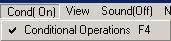
When checked, most operations (when possible) will be conditional on the color channel selection and/or masking. This is always on at startup. "Cond( On)" as opposed to "Cond(Off)" appears in the menu bar. Use F4 key to toggle.
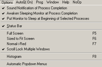
When checked, a WAV file is played when an operation is completed. The user must supply the WAV file, rename it sar.wav, and place it in the same directory as sar.exe.

The first pane shows the image dimensions. The second pane shows the color space. The third pane shows the active color channels. The fourth pane shows which layer is on top. The fifth pane shows left click pixel information. Also, the fifth plane displays information for Batch Operation, Sequential Load, and Iterated Function systems. The sixth pane gives the time that it took to complete the last operation and a progress bar for resize operations.
Pressing F5 toggles full screen on and off. With F6 and F9, useful for slide shows.
Set so that image display is resized to fit the client area of the screen. This only affects the display and not the image. The interpolation method can be selected in the Properties Dialog, which can be invoked by holding down the Ctrl key while clicking menu item. Microsoft's "Halftone" method is fastest; however, I have noticed that results differ between Windows XP and ME. "Show Combined," "Show Difference" and F7 (below) are not compatible with Halftone, but are compatible with the other methods. None are compatible with "Show Masked Area," "Show Unmasked Area," and "Show Bottom Layer Through Mask."
Tip: Before downsizing an image, incrementally sharpen images while inspecting results with this display option.
Pressing F7 displays R, G, and B channels as grey scale. Useful for examining noise in RGB channels.
Only works with JPG, PNG, and FITS.
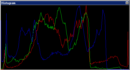
An image histogram is a graph with abscissa denoting pixel intensity and ordinate denoting the frequency of occurrence. The SAR histogram may differ from histograms of other programs in several ways. In SAR, clipped values are not shown. For example, in SAR, RGB values less than zero and greater than 255 do not appear, but, in other histograms, may appear as respective values, zero and 255. Adding/subtracting a positive constant from a color channel of an image will shift its histogram to the right/left. Multiplying/dividing a color channel by a constant greater than one will expand/contract the histogram about zero.
Also, the SAR histogram depends on color space selection. For example, in HSV mode, the H channel is shown in red, the S channel in green, and the V channel in blue.
With this option set, a menu will appear as soon as the mouse cursor hovers over a menu bar item. (I also wanted the menu to disappear as soon as the cursor is placed off the menu, but that is beyond my Windows programming skills.)
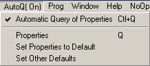
When this menu item is checked, the properties dialog will automatically appear before an operation to allow adjustment of parameter values. The default is checked.
A single dialog box gives the user access to almost all parameters. These parameters are saved in the sar.ini file when SAR closes and loaded the next time SAR opens. Clicking on a tree item on the left side of the dialog box will bring up an associated list of parameters and "combo" edit boxes on the right. Upon opening, the current value of the parameter will be displayed in an edit box. When the user enters a selection into the edit box, that selection does not take effect until the user activates the OK button or when another tree selection is made. If an entry is improper, e.g., outside allowable limits, the old parameter value will be retained. Often, values are not limited to those that appear in the drop down list under the edit box. To inspect whether your entry was accepted, without closing the dialog box, click on another tree item and then click back.
Sets dialog box properties, with the exception of registration key code, to default values.
Sets color space to RGB with all channels checked, 2nd Layer off, mask off, paint off, and Conditional on. This action is recordable and should be used to initialize some programmed actions in order to prevent the program from toggling the aforementioned items to the wrong states.
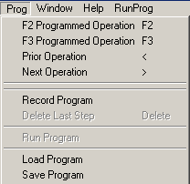
These menu items represent the F2 and F3 keys. The name of the operation programmed into the F2/F3 keys replaces "NoOp" on the menu bar. Almost any operation can be programmed into F2 by holding down the Ctrl key while clicking on the associated menu item.
After programming F2/F3 key for more than one operation, you can return to earlier operations by using >, and < (period and comma) keys. The names appear in the menu bar. Note, if the parameters for a restored operation have been changed, the previous parameters associated with the operation will not be automatically restored.
While checked, operations performed by pressing the F2 and F3 keys, along with associated parameters, are recorded. Upon unchecking, the dialog box will appear showing up to 32 recorded actions. (There is nothing to enter.) If Cancel is pressed, recording will continue. If OK is pressed, recording will stop, this menu item will be unchecked, and F2 will be programmed to run the recorded actions.
Deletes last action in recording while recording.
Runs recorded actions. Operation can be programmed into F2 key by holding down Ctrl key while clicking on this menu item.
Loads previously saved file with extension .sar.
Saves recorded steps to file with extension .sar.
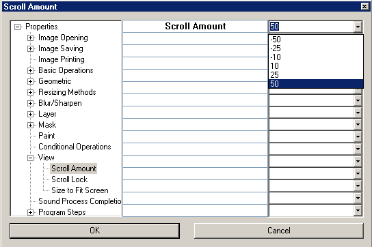
The Home key centers the image. Ctrl+Arrow keys translates image within buffer (canvas) in top layer. When the image extends beyond the border of the buffer (canvas), it wraps around to the other side. That way nothing is lost if the image is translated back to its original position. Shift+Arrow keys translates image in bottom layer." Use F10 to dismiss a menu. Use Break key to abort resize operations.
1. Under Windows ME (and probably 98), the cursor does not change for Paint. The cursor should change from an arrow to a circle with a dot at the center. This cursor is dynamically created so that the diameter of the circle can be controlled with the numeric keypad + and - keys.
2. Under Windows ME (and probably 98), the image may not be displayed in the preview window of the Print Page Setup Dialog Box. This does not affect printing.
3. Under Windows XP, if the program loses focus while processing an image, the status bar, including the progress bar, display fails to update. Also, this can occur after coming out of a screensaver or monitor sleep. This, in combination with a blank white SAR window, see 9. below, has led some people to incorrectly believe that SAR has crashed. The progress bar display (but not white screen) problem can be remedied by running SAR in XP's Win 98 compatibility mode, which is recommended.
4. The Break key remains active, if the program does not have focus.
5. Regarding the Help menu's "SAR Home Page" and "Online Manual," they may produce extraneous characters in your browser's address window, but I am uncertain of the circumstances. Of course, if this occurs, you need to remove these characters to get to the correct address.
6. With previous version 2.0, for sufficiently large images, Save As failed. Also, Open failed for sufficiently large image files. With version 2.01, these problems have been fixed with JPEG only. Save very large images as JPEG.
7. Version 2.01's RAM efficiency, for enlargement operations without floating point buffers, has been improved over version 2.0's. Per 6 above, very large images should be saved as JPEG.
8. The XP task manager may be very slow to End Task while SAR is processing an image. The Windows Me task manager is more responsive. Use Break key for resize operations when possible.
9. SAR's display of image cannot refresh itself while processing, i.e., while the cursor is an hour glass. For example, if you open Notepad in front of SAR and then close or move the notepad window, its image will remain displayed on top of SAR. Another example is when the monitor comes out of screensaver or sleep mode, the SAR window will be white. This is not a bug! At the end of processing, when the cursor is no longer an hour glass, the result will be properly displayed. Some people even thought SAR had crashed. I never anticipated that anyone would be disturbed by this. The reason that the SAR does not refresh images while processing is that the original image is no longer held in RAM. That RAM is utilized for calculations.
10. Enlargement Size Limits - Below are results from my system with 786 MB RAM and Windows XP Home Edition. These are not guaranteed size limits, but merely comprise a report of size limits on my system. Also, the maximum size that can be loaded and saved, without floating point buffers, with the exception of JPEG, is around 89 megapixels. For JPEG, this limit is around 200 megapixels. I also have Windows Me in a dual boot configuration. For Windows ME, the size limits without a floating point buffer are much smaller, but I haven't had time for extensive testing.
A few people, with Windows XP Professional Edition, have reported smaller size limits. I previously believed that low RAM was the cause, but, now, it is my understanding that each process in XP uses a maximum of 2 GB RAM + Virtual Memory. Thus, the only effect of adding more RAM is to replace virtual memory and, thereby, increase the speed of processing. With SAR 2.02, I have eliminated all messages that more RAM is needed.
I suspect two potential causes of the aforementioned people not being able to match my size limits. First, there may be something different about XP Professional vs. XP Home to account for this. Since I do not have XP Professional, I cannot duplicate their failures. Second, I have discovered that using the file opening dialog can unexpectedly fragment memory. This memory fragmentation manifests itself as a reduction of the maximum possible size of device independent bitmaps (DIB). SAR holds images in a DIB for certain operations such as printing and reading and writing certain image file formats using Microsoft code. With SAR v. 2.02, I have included a diagnostic tool for determining the maximum possible DIB size, Help>Diagnostic Tools>Maximum Dib Size. Usually, the reduction in max. pos. DIB size caused by the file open dialog is slight, but, for certain file names in certain directories, the reduction can be as much as 36%. Furthermore, the amount of fragmentation depends on whether the dialog box is closed by clicking the OK button or double clicking the file name. In my tests, it was better to double click the file name, but my tests were too few to be conclusive. Fragmentation from this source can be completely avoided by loading the image from the command line, i.e., using Windows Explorer, right click on the image file name and select "Open with SAR." Incidentally, command line loading is new with SAR v. 2.02. All results below were obtained by loading from the command line.
|
|
|
| Image Size | Max Dib Size With Floating Point Buffer | Max Dib Size Without Floating Point Buffer |
